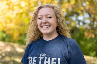
Come as you are.
Become who you're called to be.
At Bethel, you’ll discover how you're meant to make a difference. In our welcoming, Christ-guided community, you’ll experience personal transformation and outstanding preparation for life, leadership, and your career—all to propel your life forward and fulfill your purpose.
Become A Bethel Student
Apply now
You belong at Bethel. If you're ready to see who you could become, start your free application today.
Schedule Your Visit
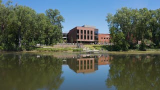
Visit Bethel
in person or online.
Experience Bethel for yourself!
Connect with us virtually or visit campus, where you'll find:
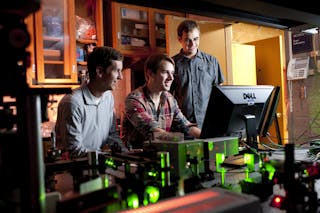
- amazing facilities and state-of-the-art labs where you’ll learn and grow
- a safe and serene campus tucked on 247 acres of wooded, lakeside property
- a great location in the heart of the Twin Cities, just 15 minutes north of St. Paul and Minneapolis
Plan your
campus visit
The best way to learn about our community is to experience it for yourself. Let us show you around!
Take a virtual tour
Before you visit, explore campus online and learn more about what day-to-day life at Bethel looks and feels like.
Upcoming events

BU Preview Day
April 26
At Bethel, you'll find a school where you belong—and you can see it for yourself by attending a Preview Day! You and your family will be able to tour campus, attend Chapel, eat in the Monson Dining Center, meet with staff and faculty, and explore areas of interest.

Summer camps at Bethel
Various dates
Experience Bethel through a variety of summer programming opportunities available to students through grade 12. Options include sports camps, arts and academic camps like Bethel Business Academy, and Living the Questions Youth Theology Institute.

Minnesota Private Colleges Week
9:30-11:30 a.m. June 24-28
You have a great chance to jumpstart your college search this summer. You can visit 17 college campuses—including Bethel—during Minnesota Private Colleges Week. Explore Bethel through campus tours and informational meetings that will be a great first step in your college search.
Transformational Academics
Explore our programs
No matter where you are in your journey, Bethel has a program to propel your life and career forward. You’ll find associate, bachelor’s, master’s, and doctoral degree offerings in more than 100 areas of study, including business, healthcare, and education.
Undergrad
Majors and minors in engaging subjects that stretch and challenge recent high school grads.
Adult Undergrad
Undergraduate programs—most of which are fully online—designed for adults looking to complete or begin their college degree.
Graduate
Advanced degree programs that prepare professionals for meaningful work in their careers and communities.
PSEO/Early College
Programs that help students get a head start on their college degree while completing high school requirements.
Seminary
Graduate programs that develop leaders for service in theological, pastoral, and ministry settings.
BUILD Program
A supportive and comprehensive educational experience for individuals with intellectual disabilities.
Find your major or program

Tuition and Financial Aid
Affordability and outcomes
We strive to make your education affordable. On average, new undergraduate students receive enough financial aid to bring the total cost per year down to about $24,000—and that number hasn’t really changed in over a decade.
Our 50,000+ alumni are tech innovators, doctors, lawyers, Emmy award-winners, pastors, state supreme court justices, and sports executives who address some of the world's greatest challenges. Let's talk details so you can join them.
100%
incoming students who receive financial aid
97%
recent graduates are employed or in graduate school
#1
highest return on investment after 10 years among Christian College Consortium schools
- Georgetown University Center on Education and the WorkforceFaith at Bethel
Guided by Christ
At Bethel, faith is infused in all we do and in every program, from business to biology. Christ is the compass giving our lives direction. But no matter where you come from, you’ll find a place where you belong at Bethel. Because here, we’re on a journey together.
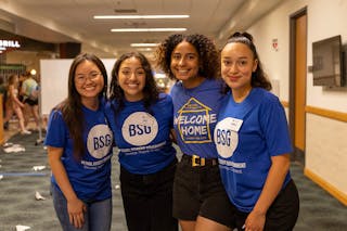
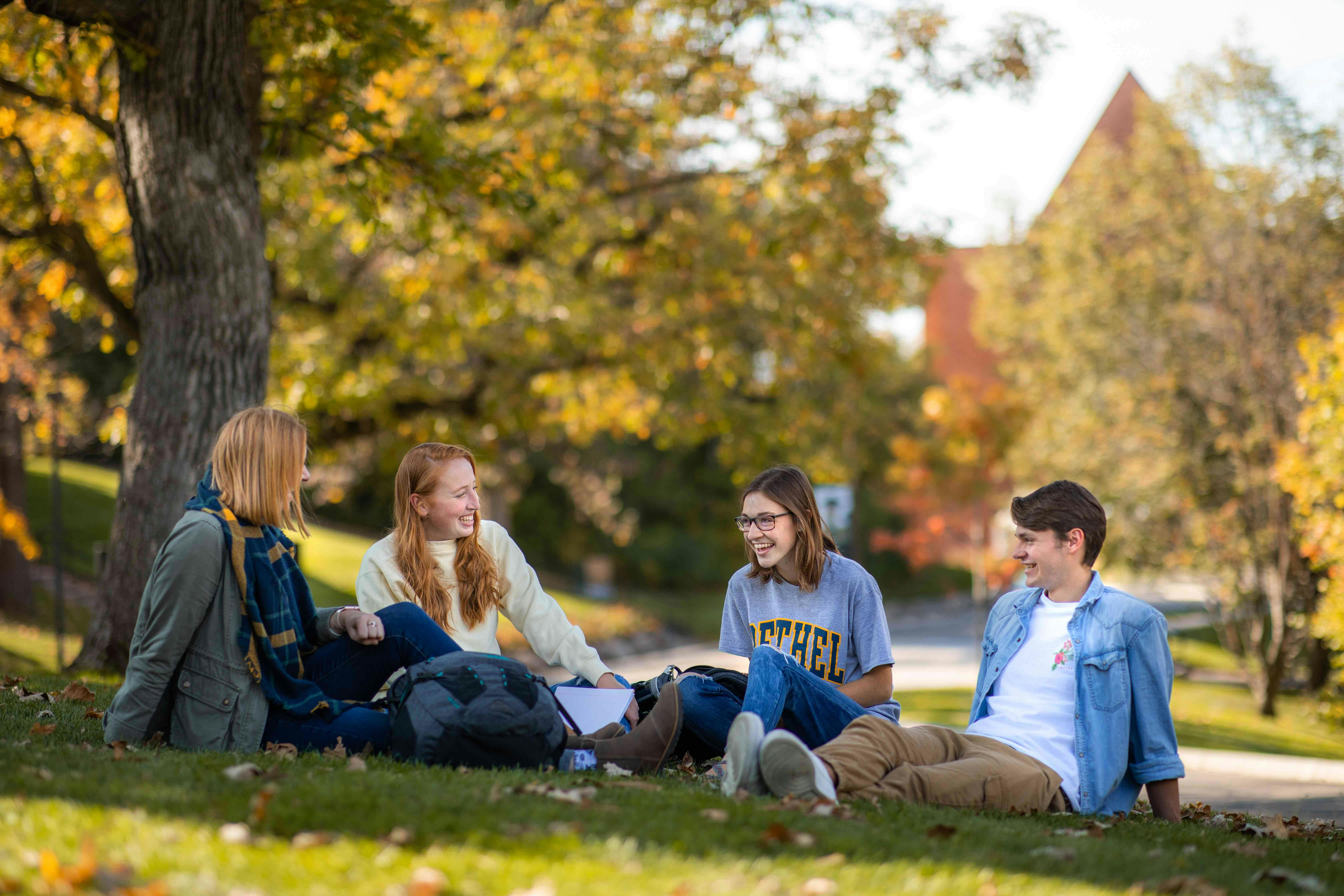
Community at Bethel
Supported by each other
At Bethel, you’ll feel at home the second you step foot on campus or connect online. You'll find a community that supports who you're becoming, and you'll develop your gifts to make an impact on our world. Together, we strive to do big things—and they’re bigger because we don’t have to do them alone.


Recent news

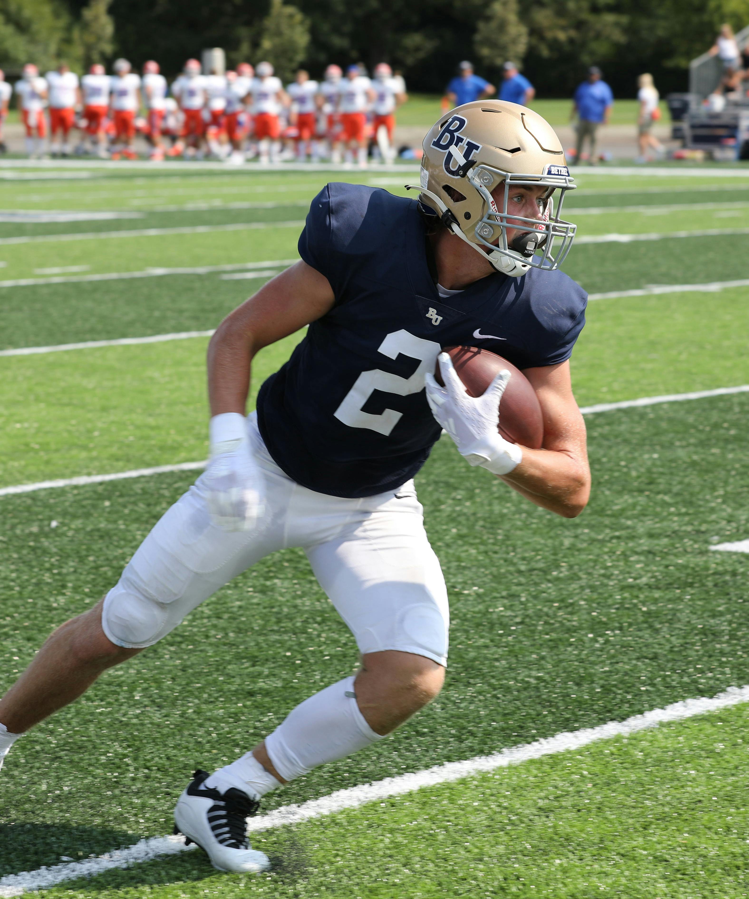
Lessons learned in sports
May 02, 2024 | 10:30 p.m.
Bill Kinney: Math professor, video producer, YouTube influencer
April 19, 2024 | Noon

Advancing healthcare: this year’s Innovation Scholars in focus
April 18, 2024 | 3 p.m.
Events
MAY 15 2024
MAY 16 2024
MAY 16 2024
English and Journalism (E&J) Celebration
4:45 p.m. Eastlund Room
Celebrate story (and meet friends old and new) at the English and Journalism spring celebration.
MAY 17 2024
Latest blog posts


Visit
Why Bethel? See for yourself. Join us for a campus visit or sign up for an online info session and get to know our exciting community.
Inquire
Want to learn more about what Bethel has to offer? We're happy to get you the information you need.